Fitxer:Symmetricwave2.png

Mida d'aquesta previsualització: 800 × 599 píxels. Altres resolucions: 320 × 240 píxels | 640 × 479 píxels | 1.024 × 767 píxels | 1.280 × 958 píxels | 1.811 × 1.356 píxels.
Fitxer original (1.811 × 1.356 píxels, mida del fitxer: 540 Ko, tipus MIME: image/png)
| Aquest fitxer i la informació mostrada a continuació provenen del dipòsit multimèdia lliure Wikimedia Commons. |

|
Aquesta imatge (de tipus physics) s'hauria de tornar a crear utilitzant gràfics vectorials com ara un fitxer SVG. Això té diversos avantatges; en trobareu més informació a Commons:Media for cleanup. Si ja disposeu d'una versió d'aquesta imatge en format SVG, us preguem que la pengeu; després, reemplaceu aquesta plantilla amb la plantilla {{Vector version available|nom nou de la imatge.svg}} en aquesta imatge.
|
Resum
| Descripció |
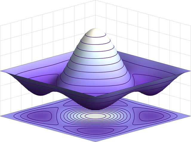
English: Symmetric wavefunction for a (bosonic) 2-particle state in an infinite square well potential. |
| Font | Treball propi |
| Autor | TimothyRias |
Llicència
Jo, el titular dels drets d'autor d'aquest treball, el public sota la següent llicència:
Aquest fitxer està subjecte a la llicència de Creative Commons Reconeixement 3.0 No adaptada.
- Sou lliure de:
- compartir – copiar, distribuir i comunicar públicament l'obra
- adaptar – fer-ne obres derivades
- Amb les condicions següents:
- reconeixement – Heu de donar la informació adequada sobre l'autor, proporcionar un enllaç a la llicència i indicar si s'han realitzat canvis. Podeu fer-ho amb qualsevol mitjà raonable, però de cap manera no suggereixi que l'autor us dóna suport o aprova l'ús que en feu.
Resum
This 3D graph shows the wavefunction for the 2-particle bosonic state for the one dimensional infinite square well at the same energy as the fermionic 2-particle groundstate. (See for example D.J. Griffiths, Introduction to quantum mechanics, Prentice Hall , 1995, section 5.1.1) The picture was created using Mathematica 6.0 using the following code:
$Assumptions = {n \[Element] Integers, m \[Element] Integers};
f[n_, x_] := Sqrt[2] Sin[n \[Pi] x];
s[n_, m_] :=
 Function[{x, y}, (f[n, x] f[m, y] + f[n, y] f[m, x])/Sqrt[2]];
swave2 = Plot3D[Evaluate[-s[3, 1][x, y]], {x, 0, 1}, {y, 0, 1},
  PlotPoints -> 35,
  PlotRange -> {-2.5, 3.5},
  MeshFunctions -> {#3 &},
  MeshStyle ->
   Directive[ColorData["DeepSeaColors"][.1], Thickness[.002]],
  Mesh -> 10,
  ColorFunction -> "LakeColors",
  BoxRatios -> {1, 1, .7},
  Boxed -> False,
  Axes -> False];
sgroundplot = Plot3D[-3, {x, 0, 1}, {y, 0, 1},
  MeshFunctions -> {s[1, 3][#1, #2] &},
  Mesh -> 10,
  MeshStyle ->
   Directive[ColorData["DeepSeaColors"][.1], Thickness[.002]],
  PlotPoints -> 50,
  ColorFunction -> (ColorData["LakeColors"][(-s[1, 3][#1, #2] + 2.5)/
      6] &)];
swave3 = Show[{swave2, sgroundplot},
 PlotRange -> {{0, 1}, {0, 1}, {-3, 3}},
 Axes -> None,
 PlotRangePadding -> None,
 ImagePadding -> 1,
 FaceGrids -> {
   {{-1, 0, 0}, {Table[i, {i, 0, 1, 1/9}],
     Table[i, {i, -3, 3, 1}]}},
   {{0, -1, 0}, {Table[i, {i, 0, 1, 1/9}], Table[i, {i, -3, 3, 1}]}}
   },
 ViewPoint -> 1000 {5, 5, 2},
 ViewVertical -> {0, 0, 1},
 ViewCenter -> {.5, .5, 0},
 ImageSize -> 600]
Export["Symmetricwave2.png", swave3, "PNG"]
Historial del fitxer
Cliqueu una data/hora per veure el fitxer tal com era aleshores.
| Data/hora | Miniatura | Dimensions | Usuari/a | Comentari | |
|---|---|---|---|---|---|
| actual | 17:52, 19 feb 2024 | | 1.811 × 1.356 (540 Ko) | Jähmefyysikko | Antialiasing and higher resolution |
| 15:18, 15 oct 2008 |  | 600 × 450 (79 Ko) | TimothyRias | {{Information |Description= |Source= |Date= |Author= |Permission= |other_versions= }} Category:Physics plots | |
| 16:52, 7 oct 2008 |  | 360 × 286 (25 Ko) | TimothyRias | {{Information |Description={{en|1=Symmetric wavefunction}} |Source=Own work by uploader |Author=TimothyRias |Date= |Permission= |other_versions= }} <!--{{ImageUpload|full}}--> |
Ús del fitxer
La pàgina següent utilitza aquest fitxer:
Ús global del fitxer
Utilització d'aquest fitxer en altres wikis:
- Utilització a ar.wikipedia.org
- Utilització a ast.wikipedia.org
- Utilització a da.wikipedia.org
- Utilització a en.wikipedia.org
- Utilització a eu.wikipedia.org
- Utilització a fa.wikipedia.org
- Utilització a ga.wikipedia.org
- Utilització a hy.wikipedia.org
- Utilització a ja.wikipedia.org
- Utilització a ko.wikipedia.org
- Utilització a pa.wikipedia.org
- Utilització a pl.wikipedia.org
- Utilització a ro.wikipedia.org
- Utilització a ru.wikipedia.org
- Utilització a sr.wikipedia.org
- Utilització a th.wikipedia.org
- Utilització a uk.wikipedia.org
- Utilització a uz.wikipedia.org
- Utilització a www.wikidata.org
- Utilització a zh-yue.wikipedia.org
- Utilització a zh.wikipedia.org