Usuari:AMontes/Polinomi

Polinomi

El gràfic d'una funció polinòmica de grau 3

En matemàtiques, un polinomi és una expressió que consisteix en variables (o indeterminades) i coeficients, que només impliquen les operacions de suma, resta, multiplicació, i exponents enters no negatius de les variables. Un exemple d'un polinomi d'una sola indeterminada x és x² − 4x + 7. Un exemple en tres variables és x³ + 2xyz² − yz + 1.

Els polinomis apareixen en una àmplia varietat d'àrees de matemàtiques i ciències. Per exemple, s'utilitzen per formar equacions polinòmiques, que codifiquen una àmplia gamma de problemes, des de problemes de paraules a problemes complexos en les ciències; S'utilitzen per definir funcions polinòmiques, que apareixen en configuracions que van des de química bàsica i física fins a economia i ciències socials; S'utilitzen en càlcul i anàlisi numèrica per aproximar altres funcions. En matemàtiques avançades, els polinomis s'utilitzen per construir anells polinòmics i varietats algebraiques, conceptes centrals en àlgebra i geometria algebraica.

Etimologia

La paraula polinomi prové de dues arrels diferents: la paraula grega "poly", que significa molts, i la paraula llatina "nomen" que significa nom. Es va derivar del terme binomial substituint l'arrel llatina bi- per la grega poly-. La paraula polinomi es va usar per primera vegada al segle XVII [1].

Notació i terminologia

La x que apareix en un polinomi es denomina habitualment una variable o indeterminada. Quan el polinomi es considera una expressió, x és un símbol fix que no té cap valor (el seu valor és "indeterminat"). Per tant, és més correcte anomenar-la una indeterminada. No obstant això, quan es considera la funció definida pel polinomi, llavors x representa l'argument de la funció i, per tant, es denomina variable. Molts autors utilitzen aquestes dues paraules indistintament.

Molts autors fan servir lletres majúscules per a les indeterminades i les minúscules corresponents per a les variables (arguments) de la funció associada. ,

Pot ser confús que un polinomi P en la indeterminada x pugui aparèixer en les fórmules com P o com P (x). .

Normalment, el nom del polinomi és P, no P(x). No obstant això, si un denota a un nombre, una variable, un altre polinomi, o, més generalment, qualsevol expressió, llavors P(a) denota, per convenció, el resultat de substituir x per a en P. Així, el polinomi P defineix la funció

$a\mapsto P(a),$

que és la funció polinòmica associada a P.

Una convenció habitual, és considerar que a és un número. Tanmateix, es pot utilitzar en qualsevol domini on es defineixin l'addició i la multiplicació (qualsevol anell). En particular, quan a és la indeterminada x, llavors la imatge de a per aquesta funció és el propi polinomi P (substituir x per x no canvia res). En altres paraules,

$P(x)=P.$

Aquesta igualtat permet escriture sigui P (x) sigui un polinomi enlloc de dir sigui P un polinomi en la indeterminada x. D'altra banda, quan no cal subratllar el nom de la indeterminada, moltes fórmules són molt més senzilles i més fàcils de llegir si els noms de les indeterminades no apareixen cada vegada que anomenem el polinomi.

Definició

Un polinomi és una expressió formada a partir de constants i simbols anomenats variables o indeterminades mitjançant suma, multiplicació i exponenciació amb potencies enteres no negatives. Es considera que dues d'aquestes expressions que es puguin transformar la una en l'altre mitjançant les propietats habituals commutativa, associativa i distributiva de la suma i multiplicación defineixen el mateix polinomi.

Un polinomi en una única variable $x$ sempre es pot escriure (o reescriure) en la forma

$a_{n}x^{n}+a_{n-1}x^{n-1}+\dotsb +a_{2}x^{2}+a_{1}x+a_{0},$

on $a_{0},\ldots ,a_{n}$ són constants and $x$ és la variable. La paraula "indeterminada" significa que $x$ no repesenta cap valor particular, podent-se substituir per qualsevol valor. L'aplicació que associa a $x$ el resultat de la substitució és una funció, denominada funció polinòmica.

L'expressió anterior pot escriure's de forma més concisa emprant notació sumatori:

$\sum _{k=0}^{n}a_{k}x^{k}$

És a dir, totot polinomi diferent de zero es pot escriure com la suma d'un nombre finit de termes. Cada terme consisteix en el producte d'un número anomenat coeficient del terme i un nombre finit de variables elevades a potències enteres no negatives. El coeficient d'un terme pot ser qualsevol número d'un conjunt especificat. Si aquest conjunt és el conjunt dels nombres racionals, parlem de "polinomis sobre els racionals". . L'exponent d'una variable d'un terme s'anomena grau de la variable en aquest terme. El grau del terme és la suma dels graus de les variables del terme, i el grau d'un polinomi és el grau més gran de qualsevol terme amb coeficient diferent de zero. Tenint en compte que $x=x^{1}$, el grau d'una variable sense exponent escrit és un.

Un terme d'un polinomi sense indeterminades és una constant o respectivament, un terme constantl o un polinomi constant. El grau d'una constant o d'un terme constant different de 0 és 0. El grau del polinomi 0 es considera generalment indefinit (però vegeu més endavant).

Per exemple: $-5x^{2}y$ és un terme. El coeficient és −5, les indeterminades son $x,y$, el grau de '$x$ és dos, mentre que el grau de '$y'$ és un. El grau del terme és la suma dels graus de les indeterminades, i per tant és 2 + 1 = 3.

La suma d'un conjunt de termes és un polinomi. Aix tenim, per exemple, el polinomi següent:

$\underbrace {_{\,}3x^{2}} _{\begin{smallmatrix}\mathrm {term} \\\mathrm {1} \end{smallmatrix}}\underbrace {-_{\,}5x} _{\begin{smallmatrix}\mathrm {term} \\\mathrm {2} \end{smallmatrix}}\underbrace {+_{\,}4} _{\begin{smallmatrix}\mathrm {term} \\\mathrm {3} \end{smallmatrix}}.$

Té tres termes: el primer és de grau dos, el segon de grau 1, i el tercer de grau 0.

Plantilla:Ancla Els polinomis de graus petits reben noms específics. Un polinomi de grau zero és un polinomi constant o simplement una constant. Els polinomis de graus un, dos o tres són polinomis lineals, quadratics i cubics respectivament. Per graus més elevats no s'acostuma a donar-los noms específics, si be de vegades els polinomis de graus quatre i cinc s'anomenen polinomis quartics i quintics. Els noms dels graus es poden aplicar tant als polinomis com als seus termes. Per example, a x² + 2x + 1 el terme 2x és el terme lineal d'un polinomi quadratic.

Plantilla:Ancla El polinomi 0, que no té cap terme, s'anomena polinomi zero. A diferència dels altres polinomis constants, el seu grau no és zero. El seu grau pot considerar-se o be indefinit o considerar que te grau negatiu (ja sigui −1 o −∞). Aquesta convenció és útil quen es defineix la Divisió Euclidiana de polinomis. El polinomi nul també és únic ja que és l'únic polinomi que té infinites arrels. El gràfic del polinomi zero és f(x) = 0, l'eix X.

Pels polinomis en més d'una variable, es diu que un polinomi és homogeni de

Plantilla:Actual si tots els termes no-nuls tenen Plantilla:Actual. El polinomi zero és homogeni, i, en tant que polinomi homogeni, el seu grau no està definit. Per example, x3y2 + 7x2y3 − 3x5 és homogeni de grau 5. Per més detalls, veure polinomi homogeni.

Per reordenar els termes en qualsevol ordre considerat es pot utilitzar la propietat commutativa de la suma. Els polinomis d'una sola variables s'odenen habitualment seguitn el seu ordre, ja sigui en "ordre descendent de les potències de x", posant en primer lloc el terme de grau més alt, o en "ordre ascendenrt de les potències de x". El polinomi de l'exemple anterior està donat en ordre descendent de x. El primer terme té coeficient 3, variable x, i exponent 2. El segon terme, te coeficient Plantilla:Actual. El tercer terme és constant.

Two terms with the same indeterminates raised to the same powers are called "similar terms" or "like terms", and they can be combined, using the distributive law, into a single term whose coefficient is the sum of the coefficients of the terms that were combined. It may happen that this makes the coefficient 0. Polynomials can be classified by the number of terms with nonzero coefficients, so that a one-term polynomial is called a monomial, a two-term polynomial is called a binomial, and a three-term polynomial is called a trinomial. The term "quadrinomial" is occasionally used for a four-term polynomial.

A real polynomial is a polynomial with real coefficients. The argument of the polynomial is not necessarily so restricted, for instance the s-plane variable in Laplace transforms. A real polynomial function is a function from the reals to the reals that is defined by a real polynomial.

A polynomial in one indeterminate is called a univariate polynomial, a polynomial in more than one indeterminate is called a multivariate polynomial. A polynomial with two indeterminates is called a bivariate polynomial. These notions refer more to the kind of polynomials one is generally working with than to individual polynomials; for instance when working with univariate polynomials one does not exclude constant polynomials (which may result, for instance, from the subtraction of non-constant polynomials), although strictly speaking constant polynomials do not contain any indeterminates at all. It is possible to further classify multivariate polynomials as bivariate, trivariate, and so on, according to the maximum number of indeterminates allowed. Again, so that the set of objects under consideration be closed under subtraction, a study of trivariate polynomials usually allows bivariate polynomials, and so on. It is common, also, to say simply "polynomials in x, y, and z", listing the indeterminates allowed.

The evaluation of a polynomial consists of substituting a numerical value to each indeterminate and carrying out the indicated multiplications and additions. For polynomials in one indeterminate, the evaluation is usually more efficient (lower number of arithmetic operations to perform) using Horner's method:

$(((\dotsb ((a_{n}x+a_{n-1})x+a_{n-2})x+\dotsb +a_{3})x+a_{2})x+a_{1})x+a_{0}.$

Arithmetic

Polynomials can be added using the associative law of addition (grouping all their terms together into a single sum), possibly followed by reordering, and combining of like terms. For example, if

${\begin{aligned}P&=3x^{2}-2x+5xy-2\\Q&=-3x^{2}+3x+4y^{2}+8\end{aligned}}$

then

$P+Q=3x^{2}-2x+5xy-2-3x^{2}+3x+4y^{2}+8$

which can be simplified to

$P+Q=x+5xy+4y^{2}+6$

To work out the product of two polynomials into a sum of terms, the distributive law is repeatedly applied, which results in each term of one polynomial being multiplied by every term of the other. For example, if

${\begin{aligned}\color {Red}P&\color {Red}{=2x+3y+5}\\\color {Blue}Q&\color {Blue}{=2x+5y+xy+1}\end{aligned}}$

then

${\begin{array}{rccrcrcrcr}{\color {Red}{P}}{\color {Blue}{Q}}&{=}&&({\color {Red}{2x}}\cdot {\color {Blue}{2x}})&+&({\color {Red}{2x}}\cdot {\color {Blue}{5y}})&+&({\color {Red}{2x}}\cdot {\color {Blue}{xy}})&+&({\color {Red}{2x}}\cdot {\color {Blue}{1}})\\&&+&({\color {Red}{3y}}\cdot {\color {Blue}{2x}})&+&({\color {Red}{3y}}\cdot {\color {Blue}{5y}})&+&({\color {Red}{3y}}\cdot {\color {Blue}{xy}})&+&({\color {Red}{3y}}\cdot {\color {Blue}{1}})\\&&+&({\color {Red}{5}}\cdot {\color {Blue}{2x}})&+&({\color {Red}{5}}\cdot {\color {Blue}{5y}})&+&({\color {Red}{5}}\cdot {\color {Blue}{xy}})&+&({\color {Red}{5}}\cdot {\color {Blue}{1}})\end{array}}$

which can be simplified to

$PQ=4x^{2}+21xy+2x^{2}y+12x+15y^{2}+3xy^{2}+28y+5$

Polynomial evaluation can be used to compute the remainder of polynomial division by a polynomial of degree one, because the remainder of the division of f(x) by (x − a) is f(a); see the polynomial remainder theorem. This is more efficient than the usual algorithm of division when the quotient is not needed.

• A sum of polynomials is a polynomial.
• A product of polynomials is a polynomial.
• A composition of two polynomials is a polynomial, which is obtained by substituting a variable of the first polynomial by the second polynomial.
• The derivative of the polynomial a_nxⁿ + a_n−1xⁿ⁻¹ + ... + a₂x² + a₁x + a₀ is the polynomial na_nxⁿ⁻¹ + (n−1)a_n−1xⁿ⁻² + ... + 2a₂x + a₁. If the set of the coefficients does not contain the integers (for example if the coefficients are integers modulo some prime number p), then ka_k should be interpreted as the sum of a_k with itself, k times. For example, over the integers modulo p, the derivative of the polynomial x^p + 1 is the polynomial 0.
• A primitive integral or antiderivative of the polynomial a_nxⁿ + a_n−1xⁿ⁻¹ + ... + a₂x² + a₁x + a₀ is the polynomial a_nxⁿ⁺¹/(n+1) + a_n−1xⁿ/n + ... + a₂x³/3 + a₁x²/2 + a₀x + c, where c is an arbitrary constant. For instance, the antiderivatives of x² + 1 have the form 1/3x³ + x + c.

As for the integers, two kinds of divisions are considered for the polynomials. The Euclidean division of polynomials that generalizes the Euclidean division of the integers. It results in two polynomials, a quotient and a remainder that are characterized by the following property of the polynomials: given two polynomials a and b such that b ≠ 0, there exists a unique pair of polynomials, q, the quotient, and r, the remainder, such that a = b q + r and degree(r) < degree(b) (here the polynomial zero is supposed to have a negative degree). By hand as well as with a computer, this division can be computed by the polynomial long division algorithm.

All polynomials with coefficients in a unique factorization domain (for example, the integers or a field) also have a factored form in which the polynomial is written as a product of irreducible polynomials and a constant. This factored form is unique up to the order of the factors and their multiplication by an invertible constant. In the case of the field of complex numbers, the irreducible factors are linear. Over the real numbers, they have the degree either one or two. Over the integers and the rational numbers the irreducible factors may have any degree. For example, the factored form of

$5x^{3}-5$

is

$5(x-1)\left(x^{2}+x+1\right)$

over the integers and the reals and

$5(x-1)\left(x+{\frac {1+i{\sqrt {3}}}{2}}\right)\left(x+{\frac {1-i{\sqrt {3}}}{2}}\right)$

over the complex numbers.

The computation of the factored form, called factorization is, in general, too difficult to be done by hand-written computation. However, efficient polynomial factorization algorithms are available in most computer algebra systems.

A formal quotient of polynomials, that is, an algebraic fraction wherein the numerator and denominator are polynomials, is called a "rational expression" or "rational fraction" and is not, in general, a polynomial. Division of a polynomial by a number, however, yields another polynomial. For example, x³/12 is considered a valid term in a polynomial (and a polynomial by itself) because it is equivalent to (1/12)x³ and 1/12 is just a constant. When this expression is used as a term, its coefficient is therefore 1/12. For similar reasons, if complex coefficients are allowed, one may have a single term like (2 + 3i) x³; even though it looks like it should be expanded to two terms, the complex number 2 + 3i is one complex number, and is the coefficient of that term. The expression 1/(x² + 1) is not a polynomial because it includes division by a non-constant polynomial. The expression (5 + y)^x is not a polynomial, because it contains an indeterminate used as exponent.

Because subtraction can be replaced by addition of the opposite quantity, and because positive integer exponents can be replaced by repeated multiplication, all polynomials can be constructed from constants and indeterminates using only addition and multiplication.

Polynomial functions

Vegeu també: Ring of polynomial functions

A polynomial function is a function that can be defined by evaluating a polynomial. A function f of one argument is thus a polynomial function if it satisfies.

$f(x)=a_{n}x^{n}+a_{n-1}x^{n-1}+\cdots +a_{2}x^{2}+a_{1}x+a_{0}\,$

for all arguments x, where n is a non-negative integer and a₀, a₁, a₂, ..., a_n are constant coefficients.

For example, the function f, taking real numbers to real numbers, defined by

$f(x)=x^{3}-x\,$

is a polynomial function of one variable. Polynomial functions of multiple variables are similarly defined, using polynomials in multiple indeterminates, as in

$f(x,y)=2x^{3}+4x^{2}y+xy^{5}+y^{2}-7.\,$

An example is also the function $f(x)=\cos(2\arccos(x))$ which, although it does not look like a polynomial, is a polynomial function on $[-1,1]$ because for every $x$ from $[-1,1]$ it is true that $f(x)=2x^{2}-1$ (see Chebyshev polynomials).

Polynomial functions are a class of functions having many important properties. They are all continuous, smooth, entire, computable, etc.

Graphs

• 
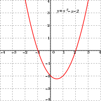  Polynomial of degree 2:
  f(x) = x² − x − 2
  = (x + 1)(x − 2)
• 
  Polynomial of degree 3:
  f(x) = x³/4 + 3x²/4 − 3x/2 − 2
  = 1/4 (x + 4)(x + 1)(x − 2)
• 
  Polynomial of degree 4:
  f(x) = 1/14 (x + 4)(x + 1)(x − 1)(x − 3)
  + 0.5
• 
  Polynomial of degree 5:
  f(x) = 1/20 (x + 4)(x + 2)(x + 1 )(x − 1)
  (x − 3)+ 2
• 
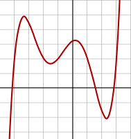
  Polynomial of degree 6:
  f(x) = 1/100 (x⁶ − 2x ⁵ − 26x⁴ + 28x³
  + 145x² - 26x - 80)
• 
  Polynomial of degree 7:
  f(x) = (x − 3)(x − 2)(x − 1)(x)(x + 1)(x + 2)
  (x + 3)

A polynomial function in one real variable can be represented by a graph.

• The graph of the zero polynomial

f(x) = 0

is the x-axis.

• The graph of a degree 0 polynomial

f(x) = a₀, where a₀ ≠ 0,

is a horizontal line with y-intercept a₀

• The graph of a degree 1 polynomial (or linear function)

f(x) = a₀ + a₁x , where a₁ ≠ 0,

is an oblique line with y-intercept a₀ and slope a₁.

• The graph of a degree 2 polynomial

f(x) = a₀ + a₁x + a₂x², where a₂ ≠ 0

is a parabola.

• The graph of a degree 3 polynomial

f(x) = a₀ + a₁x + a₂x² + a₃x³, where a₃ ≠ 0

is a cubic curve.

• The graph of any polynomial with degree 2 or greater

f(x) = a₀ + a₁x + a₂x² + ... + a_nxⁿ , where a_n ≠ 0 and n ≥ 2

is a continuous non-linear curve.

A non constant polynomial function tends to infinity when the variable increases indefinitely (in absolute value). If the degree is higher than one, the graph does not have any asymptote. It has two parabolic branches with vertical direction (one branch for positive x and one for negative x).

Polynomial graphs are analyzed in calculus using intercepts, slopes, concavity, and end behavior.

Equations

Plantilla:Main article A polynomial equation, also called algebraic equation, is an equation of the form

$a_{n}x^{n}+a_{n-1}x^{n-1}+\dotsb +a_{2}x^{2}+a_{1}x+a_{0}=0.$

For example,

$3x^{2}+4x-5=0\,$

is a polynomial equation.

When considering equations, the indeterminates (variables) of polynomials are also called unknowns, and the solutions are the possible values of the unknowns for which the equality is true (in general more than one solution may exist). A polynomial equation stands in contrast to a polynomial identity like (x + y)(x − y) = x² − y², where both expressions represent the same polynomial in different forms, and as a consequence any evaluation of both members gives a valid equality.

In elementary algebra, methods such as the quadratic formula are taught for solving all first degree and second degree polynomial equations in one variable. There are also formulas for the cubic and quartic equations. For higher degrees, the Abel–Ruffini theorem asserts that there can not exist a general formula in radicals. However, root-finding algorithms may be used to find numerical approximations of the roots of a polynomial expression of any degree.

The number of real solutions of a polynomial equation with real coefficients may not exceed the degree, and equals the degree when the complex solutions are counted with their multiplicity. This fact is called the fundamental theorem of algebra.

Solving equations

Vegeu també: Root-finding algorithm i Properties of polynomial roots

Every polynomial P in x defines a function $x\mapsto P(x),$ called the polynomial function associated to P; the equation P(x) = 0 is the polynomial equation associated to P. The solutions of this equation are called the roots of the polynomial, or the zeros of the associated function (they correspond to the points where the graph of the function meets the x-axis).

A number a is a root of a polynomial P if and only if the linear polynomial x − a divides P, that is if there is another polynomial Q such that P = (x – a) Q. It may happen that x − a divides P more than once: if (x − a)² divides P then a is called a multiple root of P, and otherwise a is called a simple root of P. If P is a nonzero polynomial, there is a highest power m such that (x − a)^m divides P, which is called the multiplicity of the root a in P. When P is the zero polynomial, the corresponding polynomial equation is trivial, and this case is usually excluded when considering roots, as, with the above definitions, every number is a root of the zero polynomial, with a undefined multiplicity. With this exception made, the number of roots of P, even counted with their respective multiplicities, cannot exceed the degree of P. The relation between the coefficients of a polynomial and its roots is described by Vieta's formulas.

Some polynomials, such as x² + 1, do not have any roots among the real numbers. If, however, the set of accepted solutions is expanded to the complex numbers, every non-constant polynomial has at least one root; this is the fundamental theorem of algebra. By successively dividing out factors x − a, one sees that any polynomial with complex coefficients can be written as a constant (its leading coefficient) times a product of such polynomial factors of degree 1; as a consequence, the number of (complex) roots counted with their multiplicities is exactly equal to the degree of the polynomial.

There may be several meanings of "solving an equation". One may want to express the solutions as explicit numbers; for example, the unique solution of 2x – 1 = 0 is 1/2. Unfortunately, this is, in general, impossible for equations of degree greater than one, and, since the ancient times, mathematicians have searched to express the solutions as algebraic expression; for example the golden ratio $(1+{\sqrt {5}})/2$ is the unique positive solution of $x^{2}-x-1=0.$ In the ancient times, they succeeded only for degrees one and two. For quadratic equations, the quadratic formula provides such expressions of the solutions. Since the 16th century, similar formulas (using cube roots in addition to square roots), but much more complicated are known for equations of degree three and four (see cubic equation and quartic equation). But formulas for degree 5 and higher eluded researchers for several centuries. In 1824, Niels Henrik Abel proved the striking result that there are equations of degree 5 whose solutions cannot be expressed by a (finite) formula, involving only arithmetic operations and radicals (see Abel–Ruffini theorem). In 1830, Évariste Galois proved that most equations of degree higher than four cannot be solved by radicals, and showed that for each equation, one may decide whether it is solvable by radicals, and, if it is, solve it. This result marked the start of Galois theory and group theory, two important branches of modern algebra. Galois himself noted that the computations implied by his method were impracticable. Nevertheless, formulas for solvable equations of degrees 5 and 6 have been published (see quintic function and sextic equation).

When there is no algebraic expression for the roots, and when such an algebraic expression exists but is too large for being useful, the unique way of solving is to compute numerical approximations of the solutions. There are many methods for that, some are restricted to polynomials and others may apply to any continuous function. The most efficient algorithms allow solving easily (on a computer) polynomial equations of degree higher than 1,000 (see Root-finding algorithm).

For polynomials in more than one indeterminate, the combinations of values for the variables for which the polynomial function takes the value zero are generally called zeros instead of "roots". The study of the sets of zeros of polynomials is the object of algebraic geometry. For a set of polynomial equations in several unknowns, there are algorithms to decide whether they have a finite number of complex solutions, and, if this number is finite, for computing the solutions. See System of polynomial equations.

The special case where all the polynomials are of degree one is called a system of linear equations, for which another range of different solution methods exist, including the classical Gaussian elimination.

A polynomial equation for which one is interested only in the solutions which are integers is called a Diophantine equation. Solving Diophantine equations is generally a very hard task. It has been proved that there cannot be any general algorithm for solving them, and even for deciding whether the set of solutions is empty (see Hilbert's tenth problem). Some of the most famous problems that have been solved during the fifty last years are related to Diophantine equations, such as Fermat's Last Theorem.

Generalizations

There are several generalizations of the concept of polynomials.

Trigonometric polynomials

Plantilla:Main article A trigonometric polynomial is a finite linear combination of functions sin(nx) and cos(nx) with n taking on the values of one or more natural numbers. The coefficients may be taken as real numbers, for real-valued functions.

If sin(nx) and cos(nx) are expanded in terms of sin(x) and cos(x), a trigonometric polynomial becomes a polynomial in the two variables sin(x) and cos(x) (using List of trigonometric identities#Multiple-angle formulae). Conversely, every polynomial in sin(x) and cos(x) may be converted, with Product-to-sum identities, into a linear combination of functions sin(nx) and cos(nx). This equivalence explains why linear combinations are called polynomials.

For complex coefficients, there is no difference between such a function and a finite Fourier series.

Trigonometric polynomials are widely used, for example in trigonometric interpolation applied to the interpolation of periodic functions. They are used also in the discrete Fourier transform.

Matrix polynomials

Plantilla:Main article A matrix polynomial is a polynomial with matrices as variables. Given an ordinary, scalar-valued polynomial

$P(x)=\sum _{i=0}^{n}{a_{i}x^{i}}=a_{0}+a_{1}x+a_{2}x^{2}+\cdots +a_{n}x^{n},$

this polynomial evaluated at a matrix A is

$P(A)=\sum _{i=0}^{n}{a_{i}A^{i}}=a_{0}I+a_{1}A+a_{2}A^{2}+\cdots +a_{n}A^{n},$

where I is the identity matrix.

A matrix polynomial equation is an equality between two matrix polynomials, which holds for the specific matrices in question. A matrix polynomial identity is a matrix polynomial equation which holds for all matrices A in a specified matrix ring M_n(R).

Laurent polynomials

Plantilla:Main article Laurent polynomials are like polynomials, but allow negative powers of the variable(s) to occur.

Rational functions

Plantilla:Main article A rational fraction is the quotient (algebraic fraction) of two polynomials. Any algebraic expression that can be rewritten as a rational fraction is a rational function.

While polynomial functions are defined for all values of the variables, a rational function is defined only for the values of the variables for which the denominator is not zero.

The rational fractions include the Laurent polynomials, but do not limit denominators to powers of an indeterminate.

Power series

Plantilla:Main article Formal power series are like polynomials, but allow infinitely many non-zero terms to occur, so that they do not have finite degree. Unlike polynomials they cannot in general be explicitly and fully written down (just like irrational numbers cannot), but the rules for manipulating their terms are the same as for polynomials. Non-formal power series also generalize polynomials, but the multiplication of two power series may not converge.

Other examples

• A bivariate polynomial where the second variable is substituted by an exponential function applied to the first variable, for example P(x, e^x), may be called an exponential polynomial.

Applications

Calculus

Vegeu també: Polynomial interpolation

The simple structure of polynomial functions makes them quite useful in analyzing general functions using polynomial approximations. An important example in calculus is Taylor's theorem, which roughly states that every differentiable function locally looks like a polynomial function, and the Stone–Weierstrass theorem, which states that every continuous function defined on a compact interval of the real axis can be approximated on the whole interval as closely as desired by a polynomial function.

Calculating derivatives and integrals of polynomial functions is particularly simple. For the polynomial function

$\sum _{i=0}^{n}a_{i}x^{i}$

the derivative with respect to x is

$\sum _{i=1}^{n}a_{i}ix^{i-1}$

and the indefinite integral is

$\sum _{i=0}^{n}{a_{i} \over i+1}x^{i+1}+c.$

Abstract algebra

Plantilla:Main article In abstract algebra, one distinguishes between polynomials and polynomial functions. A polynomial f in one indeterminate x over a ring R is defined as a formal expression of the form

$f=a_{n}x^{n}+a_{n-1}x^{n-1}+\cdots +a_{1}x^{1}+a_{0}x^{0}$

where n is a natural number, the coefficients a₀, . . ., a_n are elements of R, and x is a formal symbol, whose powers xⁱ are just placeholders for the corresponding coefficients a_i, so that the given formal expression is just a way to encode the sequence (a₀, a₁, . . .), where there is an n such that a_i = 0 for all i > n. Two polynomials sharing the same value of n are considered equal if and only if the sequences of their coefficients are equal; furthermore any polynomial is equal to any polynomial with greater value of n obtained from it by adding terms in front whose coefficient is zero. These polynomials can be added by simply adding corresponding coefficients (the rule for extending by terms with zero coefficients can be used to make sure such coefficients exist). Thus each polynomial is actually equal to the sum of the terms used in its formal expression, if such a term a_ixⁱ is interpreted as a polynomial that has zero coefficients at all powers of x other than xⁱ. Then to define multiplication, it suffices by the distributive law to describe the product of any two such terms, which is given by the rule

$ax^{k}\;bx^{l}=abx^{k+l}$

   for all elements a, b of the ring R and all natural numbers k and l.

Thus the set of all polynomials with coefficients in the ring R forms itself a ring, the ring of polynomials over R, which is denoted by R[x]. The map from R to R[x] sending r to rx⁰ is an injective homomorphism of rings, by which R is viewed as a subring of R[x]. If R is commutative, then R[x] is an algebra over R.

One can think of the ring R[x] as arising from R by adding one new element x to R, and extending in a minimal way to a ring in which x satisfies no other relations than the obligatory ones, plus commutation with all elements of R (that is xr = rx). To do this, one must add all powers of x and their linear combinations as well.

Formation of the polynomial ring, together with forming factor rings by factoring out ideals, are important tools for constructing new rings out of known ones. For instance, the ring (in fact field) of complex numbers, which can be constructed from the polynomial ring R[x] over the real numbers by factoring out the ideal of multiples of the polynomial x² + 1. Another example is the construction of finite fields, which proceeds similarly, starting out with the field of integers modulo some prime number as the coefficient ring R (see modular arithmetic).

If R is commutative, then one can associate to every polynomial P in R[x], a polynomial function f with domain and range equal to R (more generally one can take domain and range to be the same unital associative algebra over R). One obtains the value f(r) by substitution of the value r for the symbol x in P. One reason to distinguish between polynomials and polynomial functions is that over some rings different polynomials may give rise to the same polynomial function (see Fermat's little theorem for an example where R is the integers modulo p). This is not the case when R is the real or complex numbers, whence the two concepts are not always distinguished in analysis. An even more important reason to distinguish between polynomials and polynomial functions is that many operations on polynomials (like Euclidean division) require looking at what a polynomial is composed of as an expression rather than evaluating it at some constant value for x.

Divisibility

Plantilla:Main article In commutative algebra, one major focus of study is divisibility among polynomials. If R is an integral domain and f and g are polynomials in R[x], it is said that f divides g or f is a divisor of g if there exists a polynomial q in R[x] such that f q = g. One can show that every zero gives rise to a linear divisor, or more formally, if f is a polynomial in R[x] and r is an element of R such that f(r) = 0, then the polynomial (x − r) divides f. The converse is also true. The quotient can be computed using the polynomial long division.

If F is a field and f and g are polynomials in F[x] with g ≠ 0, then there exist unique polynomials q and r in F[x] with

$f=q\,g+r$

and such that the degree of r is smaller than the degree of g (using the convention that the polynomial 0 has a negative degree). The polynomials q and r are uniquely determined by f and g. This is called Euclidean division, division with remainder or polynomial long division and shows that the ring F[x] is a Euclidean domain.

Analogously, prime polynomials (more correctly, irreducible polynomials) can be defined as non-zero polynomials which cannot be factorized into the product of two non constant polynomials. In the case of coefficients in a ring, "non constant" must be replaced by "non constant or non unit" (both definitions agree in the case of coefficients in a field). Any polynomial may be decomposed into the product of an invertible constant by a product of irreducible polynomials. If the coefficients belong to a field or a unique factorization domain this decomposition is unique up to the order of the factors and the multiplication of any non unit factor by a unit (and division of the unit factor by the same unit). When the coefficients belong to integers, rational numbers or a finite field, there are algorithms to test irreducibility and to compute the factorization into irreducible polynomials (see Factorization of polynomials). These algorithms are not practicable for hand written computation, but are available in any computer algebra system. Eisenstein's criterion can also be used in some cases to determine irreducibility.

Other applications

Vegeu també: Orthogonal polynomial, B-spline, i spline interpolation

Polynomials serve to approximate other functions, such as the use of splines.

Polynomials are frequently used to encode information about some other object. The characteristic polynomial of a matrix or linear operator contains information about the operator's eigenvalues. The minimal polynomial of an algebraic element records the simplest algebraic relation satisfied by that element. The chromatic polynomial of a graph counts the number of proper colourings of that graph.

The term "polynomial", as an adjective, can also be used for quantities or functions that can be written in polynomial form. For example, in computational complexity theory the phrase polynomial time means that the time it takes to complete an algorithm is bounded by a polynomial function of some variable, such as the size of the input.

History

Plantilla:Main article Determining the roots of polynomials, or "solving algebraic equations", is among the oldest problems in mathematics. However, the elegant and practical notation we use today only developed beginning in the 15th century. Before that, equations were written out in words. For example, an algebra problem from the Chinese Arithmetic in Nine Sections, circa 200 BCE, begins "Three sheafs of good crop, two sheafs of mediocre crop, and one sheaf of bad crop are sold for 29 dou." We would write 3x + 2y + z = 29.

History of the notation

Plantilla:Main article The earliest known use of the equal sign is in Robert Recorde's The Whetstone of Witte, 1557. The signs + for addition, − for subtraction, and the use of a letter for an unknown appear in Michael Stifel's Arithemetica integra, 1544. René Descartes, in La géometrie, 1637, introduced the concept of the graph of a polynomial equation. He popularized the use of letters from the beginning of the alphabet to denote constants and letters from the end of the alphabet to denote variables, as can be seen above, in the general formula for a polynomial in one variable, where the a's denote constants and x denotes a variable. Descartes introduced the use of superscripts to denote exponents as well.

See also

• Lill's method
• List of polynomial topics
• Polynomials on vector spaces
• Power series
• Table of mathematical expressions
• Polynomial transformations
• Polynomiography

References

• Barbeau, E.J.. Polynomials. Springer, 2003. ISBN 978-0-387-40627-5. 
• Solving Polynomial Equations: Foundations, Algorithms, and Applications. Springer, 2006. ISBN 978-3-540-27357-8. 
• Cahen, Paul-Jean; Chabert, Jean-Luc. Integer-Valued Polynomials. American Mathematical Society, 1997. ISBN 978-0-8218-0388-2. 
• Plantilla:Lang Algebra. This classical book covers most of the content of this article.
• Leung, Kam-tim. Polynomials and Equations. Hong Kong University Press, 1992. ISBN 9789622092716. 
• Mayr, K. Über die Auflösung algebraischer Gleichungssysteme durch hypergeometrische Funktionen. Monatshefte für Mathematik und Physik vol. 45, (1937) pp. 280–313.
• Prasolov, Victor V. Polynomials. Springer, 2005. ISBN 978-3-642-04012-2. 
• Sethuraman, B.A.. «Polynomials». A: Rings, Fields, and Vector Spaces: An Introduction to Abstract Algebra Via Geometric Constructibility. Springer, 1997. ISBN 978-0-387-94848-5. 
• Umemura, H. Solution of algebraic equations in terms of theta constants. In D. Mumford, Tata Lectures on Theta II, Progress in Mathematics 43, Birkhäuser, Boston, 1984.
• von Lindemann, F. Über die Auflösung der algebraischen Gleichungen durch transcendente Functionen. Nachrichten von der Königl. Gesellschaft der Wissenschaften, vol. 7, 1884. Polynomial solutions in terms of theta functions.
• von Lindemann, F. Über die Auflösung der algebraischen Gleichungen durch transcendente Functionen II. Nachrichten von der Königl. Gesellschaft der Wissenschaften und der Georg-Augusts-Universität zu Göttingen, 1892 edition.

External links

A Wikimedia Commons hi ha contingut multimèdia relatiu a: AMontes/Polinomi

Vegeu AMontes/Polinomi en el Viccionari, el diccionari lliure.Viccionari

• Michiel Hazewinkel (ed.). Polynomial. Encyclopedia of Mathematics (en anglès). Springer, 2001. ISBN 978-1-55608-010-4. 
• «Euler's Investigations on the Roots of Equations». Arxivat de l'original el September 24, 2012.
• Weisstein, Eric W., «Polynomial» a MathWorld (en anglès).

Algebra de polinomis

Els coeficients d'un polinomi s'han de poder sumar, multiplicar i les operacions han de ser conmutatives i distributives. Per tant, cal que els coeficients siguin elements d'un anell  o més habitualment d'un cos (veure cos i anell).  Considerem polinomis amb coeficients en un cos: el cos $\mathbb {Q}$ dels nombres racionals, o el cos $\mathbb {R}$ dels nombres reals o el cos $\mathbb {C}$ del nombres complexos. Poden considerar-se també altres cossos, però  aquests són els més habituals. El conjunt dels polinomis sobre un cos $K$ amb variables $x_{1},\dots ,x_{n}$ es denota $K[x_{1},\dots ,x_{n}]$. Així, per exemple el polinomi $p=3x^{2}y+2xz-3$  és un polinomi de $\mathbb {Q} [x,y,z]$. Òbviament també és un polinomi de $\mathbb {R} [x,y,z]$ i de $\mathbb {C} [x,y,z]$.

Els polinomis són objectes bàsics de l'Àlgebra i la Geometria, ja que relacionen intrínsecament les dues matèries a través de les varietats i els ideals.

Definició: Sigui $K$ un cos ($\mathbb {Q}$, o $\mathbb {R}$ o $\mathbb {C}$), i siguin $f_{1},\dots ,f_{s}$ un conjunt de polinomis

de $K[x_{1},\dots ,x_{n}]$. El conjunt

$V=\mathbb {V} (f_{1},\dots ,f_{s})=\{(a_{1},\dots ,a_{n})\subset K'^{n}:f_{i}(a_{1},\dots ,a_{n})=0{\hbox{ per tot }}1\leq i\leq s\}$

és la varietat afí de  $K'^{n}$ definida per $f_{1},\dots ,f_{s}$, on $K'$ és un cos que pot ser $K$ o un cos més ampli que contingui $K$ (extensió de <math>K</math).

Per tant, la varietat af\'i $V=\mathbf {V} (f_{1},\dots ,f_{s})\subset K'^{n}$ \és el conjunt de totes les solucions del sistema d'equacions $f_{1}(x_{1},\dots ,x_{n})=\dots =f_{s}(x_{1},\dots ,x_{n})=0$, amb valors al cos $\mathbb {K'}$.

Definició: Sigui $K$ un cos ($\mathbb {Q}$, o $\mathbb {R}$ o $\mathbb {C}$), i siguin $f_{1},\dots ,f_{s}$ un conjunt de polinomis

de $K[x_{1},\dots ,x_{n}]$. El conjunt de polinomis

${\mathcal {I}}=\langle f_{1},\dots ,f_{s}\rangle =\{f\in K[x_{1},\dots ,x_{n}]:f=\sum _{i=1}^{s}g_{i}f_{i}\}$

on els $g_{i}$ són polinomis arbitraris de $K[x_{1},\dots ,x_{n}]$ és l'{\em ideal} generat per $f_{1},\dots ,f_{s}$.

Òbviament es té $\mathbf {V} (f_{1},\dots ,f_{s})=\mathbf {V} ({\mathcal {I}})$, ja que tots els polinomis de ${\mathcal {I}}$ s'anul.len a $\mathbf {V} (f_{1},\dots ,f_{s})$ i recíprocament tot zero de $\mathbf {V} ({\mathcal {I}})$ és un zero de $V$.

Axil referint-nos al polinomi de l'exemple $p=5x^{3}+5$ que descomposa en $p=5(x-1)\left(x+{\frac {1+i{\sqrt {3}}}{2}}\right)\left(x+{\frac {1-i{\sqrt {3}}}{2}}\right)$, la varietat $\mathbf {V} (p)$ a $\mathbb {C}$ és:

$\mathbf {V} (5x^{3}+5)=\left\{1,{\frac {-1-i{\sqrt {3}}}{2}},{\frac {-1+i{\sqrt {3}}}{2}}\right\}$

mentre que a $\mathbb {Q}$ o $\mathbb {R}$ seria $\mathbf {V} (p)=\{1\}$.

Un exemple de dos variables és: $f=x^{2}+2xy+y^{2}-50$, que descomposa en $f=(x-y-{\sqrt {50}})(x-y+{\sqrt {50}})$. Per tant resulta $\mathbf {V} (f)=\mathbf {V} (x-y-{\sqrt {50}})\cup \mathbf {V} (x-y-{\sqrt {50}})$. Per tant representa un parell de rectes del pla real.

L'estudi de les varietats i els ideals de polinomis multivariats dona lloc a l'Àlgebra Computacional i a la Geometria algebraica, disciplines molt extenses de les matemàtiques. Entre els mètodes que desenvolupen per analitzar els ideals i les varietats figura la base de Gröbner.